
Conditional formatting is a powerful tool in Excel that allows you to highlight cells or ranges of cells based on specific criteria.
This can help you quickly identify important data points, errors, or trends in your data. In this article, we’ll look at how to use conditional formatting in Excel and provide some examples.
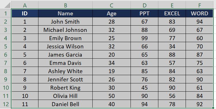
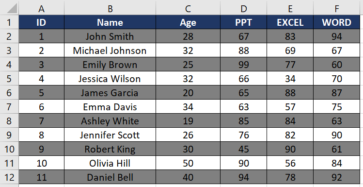
To start, let’s take a look at some data that we can use for our examples:
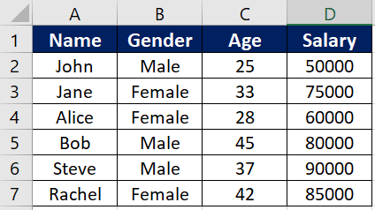
Now that we have our data, let’s explore some ways that we can use conditional formatting to highlight specific values or patterns.
Table of Contents
Highlight Cells Based on Value with Conditional formatting in Excel
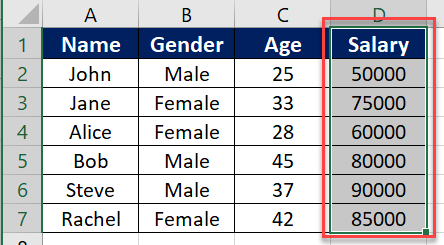
One of the simplest ways to use conditional formatting is to highlight cells that meet a certain value criteria. For example, let’s say we want to highlight all of the cells in the Salary column that are above 75000. Here’s how we would do it:
– Select the cells that you want to apply the formatting to (in this case, the cells in the Salary column).
– On the Home tab, click on the Conditional Formatting dropdown menu (it’s located in the Styles group).
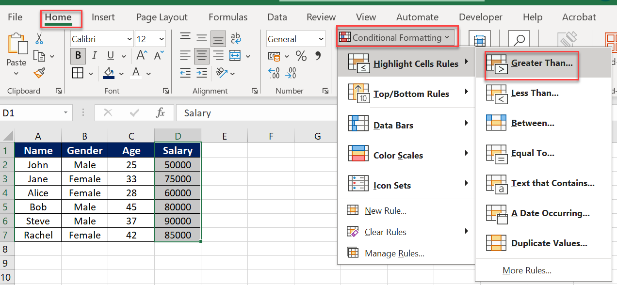
– Select Highlight Cells Rules, then choose Greater Than.
– In the dialog box that appears, enter the value that you want to compare to (in this case, 75000).
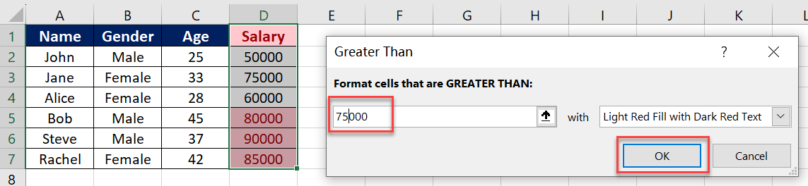
– Choose a color for the formatting (such as red).
See also: Mastering the Linux Command Line — Your Complete Free Training Guide
– Click OK.
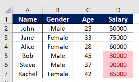
Now, all of the cells in the Salary column that are greater than 75000 will be highlighted in red.
Highlight Cells Based on Text with Conditional formatting in Excel
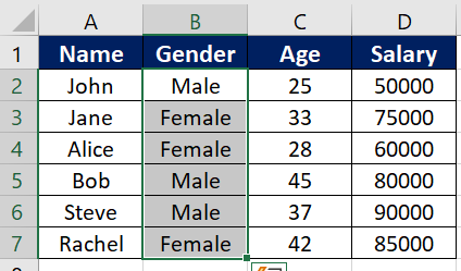
In addition to highlighting cells based on value, you can also use conditional formatting to highlight cells based on text. In our example data table above, let’s say that we want to highlight all of the female names in the first column. Here’s how we would do it:
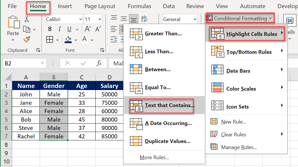
– Select the cells that you want to apply the formatting to (in this case, the cells in the Gender column).
– On the Home tab, click on the Conditional Formatting dropdown menu.
– Select Highlight Cells Rules, then choose Text that Contains.
– In the dialog box that appears, enter the text that you want to search for (in this case, “Female”).
– Choose a color for the formatting (such as yellow).
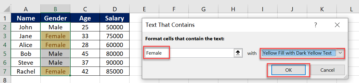
– Click OK.
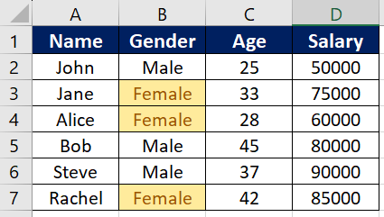
Now, all of the cells in the Name column that contain the word “Female” will be highlighted in yellow.
Highlight Alternate Rows/Columns with Conditional formatting in Excel
Another useful way to use conditional formatting is to highlight alternate rows or columns in your data table. This can help make it easier to read and identify patterns in your data. Here’s how we would do it:
– Select the cells that you want to apply the formatting to (in this case, the entire data table).
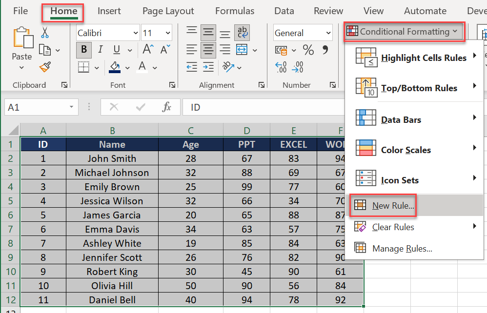
– On the Home tab, click on the Conditional Formatting dropdown menu.
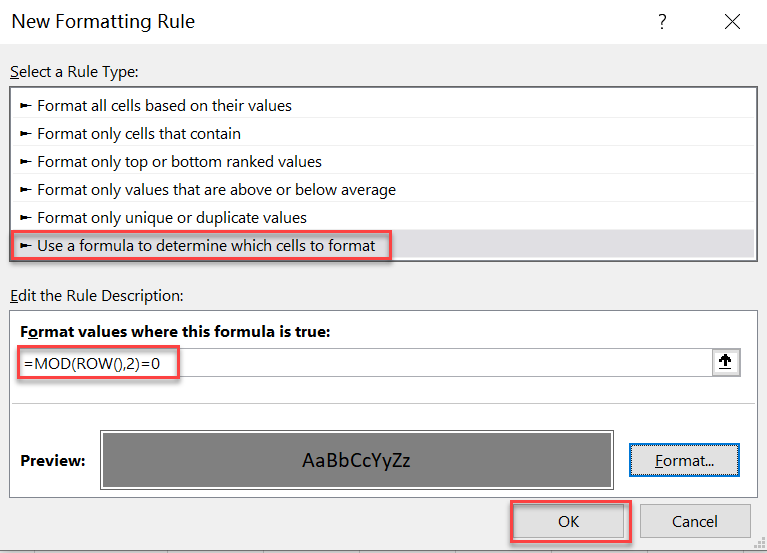
– Select New Rule, then choose Use a Formula to Determine Which Cells to Format.
– In the formula bar that appears, enter the following formula:
=MOD(ROW(),2)=0
– Choose a color for the formatting (such as light gray).
– Click OK.
Now, every other row in your data table will be highlighted in light gray.
Highlight Duplicate Values with Conditional formatting in Excel
Finally, you can use conditional formatting to highlight duplicate values in your data table. This can help you quickly identify errors or duplicates in your data. Here’s how we would do it:
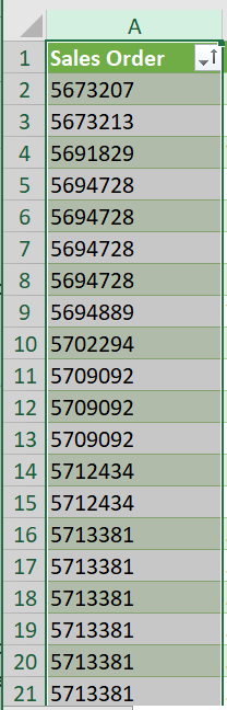
– Select the cells that you want to apply the formatting to (in this case, the cells in the Sales Order column).
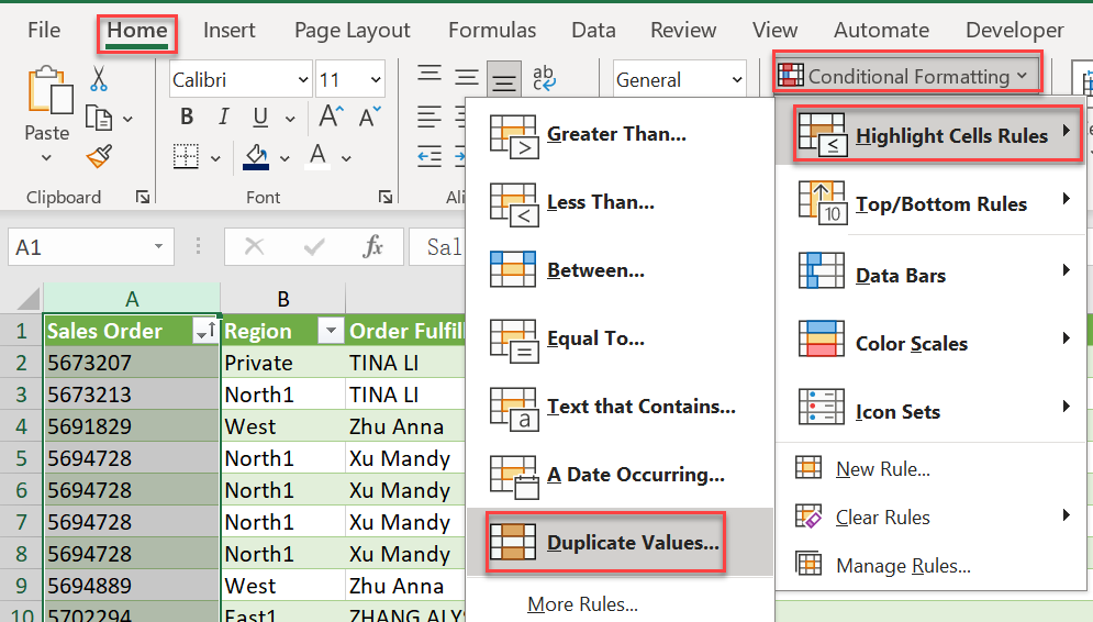
– On the Home tab, click on the Conditional Formatting dropdown menu.
– Select Highlight Cells Rules, then choose Duplicate Values.
– In the dialog box that appears, choose a color for the formatting (such as yellow).
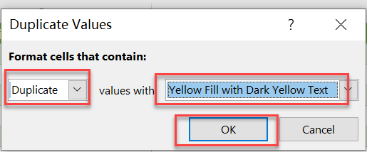
– Click OK.
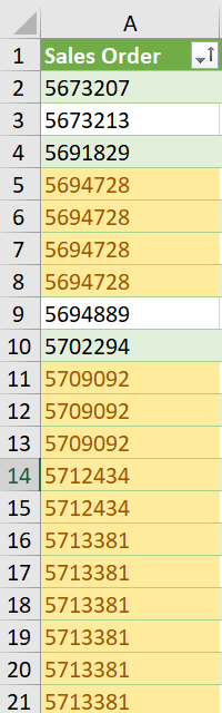
Now, any duplicate values in your data table will be highlighted in yellow.
In conclusion, conditional formatting is a powerful tool in Excel that can help you quickly identify and highlight specific values and patterns in your data.
By experimenting with different rule types and color schemes, you can make your data tables more informative and visually appealing.