Formatting in Excel is an important aspect that helps make your data more visually appealing and easier to understand.
In addition, formatting can also help improve the readability of your Excel tables. One easy way to apply formatting in Excel is by using the Ctrl+Q shortcut.
In this article, we will learn how to use formatting in Ctrl+Q in Excel tables and provide some Excel data table examples.
Table of Contents
What is formatting in Ctrl+Q?
Formatting in Ctrl+Q is a keyboard shortcut used to quickly apply formatting to cells in Excel tables.
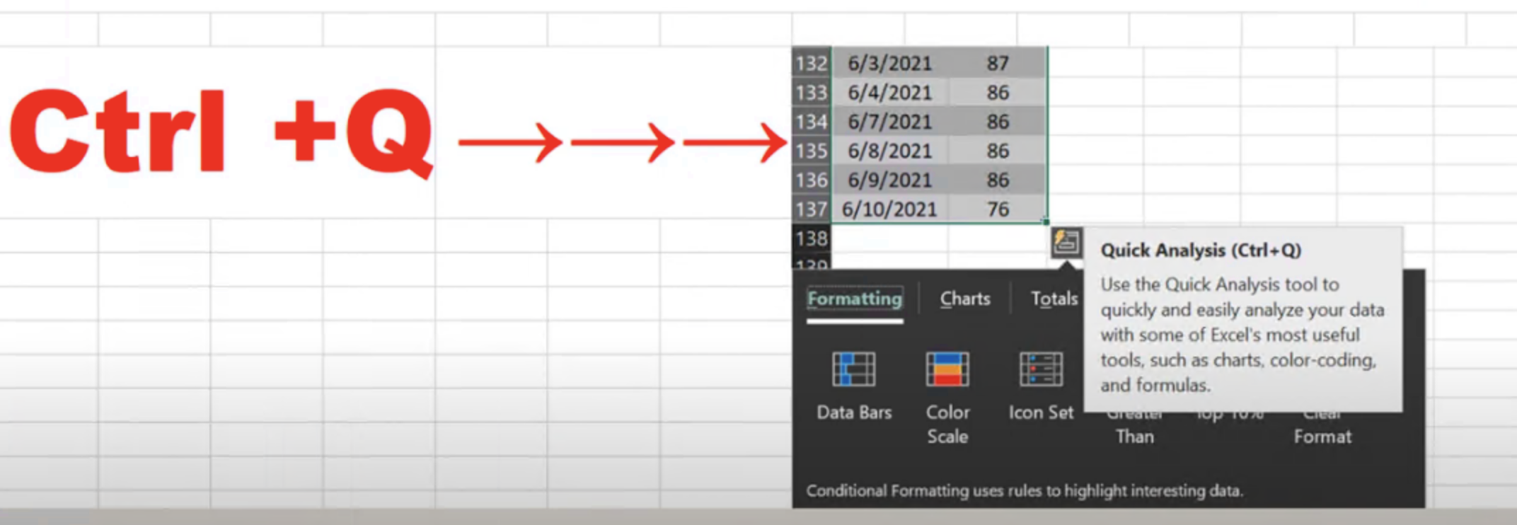
The Ctrl+Q shortcut is used to apply the default formatting styles that have been set up in your workbook.
This shortcut is a helpful tool for quickly applying formatting to your data without having to go through the tedious process of individually formatting each cell.
How to Use Formatting in Ctrl+Q
Here are the steps to use formatting in Ctrl+Q:
1. Select the cells in the table that you want to apply formatting to.
2. Once the cells are selected, press the Ctrl+Q keys simultaneously.
3. The selected cells will now have the default formatting style applied to them.
Examples
Here are some Excel data table examples with formatting applied using Ctrl+Q:
See also: Mastering the Linux Command Line — Your Complete Free Training Guide
Example 1:
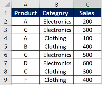
In this example, we have a table with sales data. We want to apply formatting to highlight the highest and lowest sales figures.
Select the cells that you want to apply formatting to (i.e., cells C2 to C9).
Press Ctrl+Q to apply the default formatting style.
In the Home tab, click on Conditional Formatting > Highlight Cells Rules > Greater Than.

Enter the highest sales figure (i.e., 350) in the box and choose a color to highlight the cells.


We can also set Data Bars, Color scale and Icon set as below:


Example 2:
In this example, we have a table with expenses data. We want to apply formatting to display negative numbers in red font.
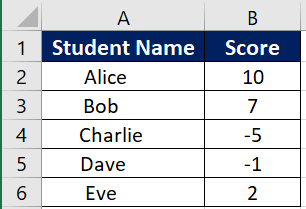
Select the cells that you want to apply formatting to (i.e., cells B2 to E6).
Press Ctrl+Q to apply the default formatting style.
In the Home tab, click on Conditional Formatting > New Rule.

Choose the option “Format only cells that contain” and change the dropdown to “Less than”.
Enter “0” in the value field.

Click on the Format button and select the Font tab.
Choose red in the Font color dropdown and click OK.
The resulting table will display the negative numbers in red font.

Conclusion
Formatting in Ctrl+Q is a useful feature that can expedite Excel data table formatting. It is important to keep in mind that formatting should aid in the interpretation of your data. By following these simple steps, you can apply professional formatting quickly and easily to enhance the visual expression of your tables.