
SUMIF is a powerful function in Microsoft Excel that allows you to sum up values in a range if they meet certain criteria.
It is particularly useful when you have large sets of data and want to identify and sum up specific values without having to do manual calculations.
Table of Contents
SUMIF Syntax in Excel
SUMIF works by taking three arguments: Range, Criteria, and Sum_Range. Syntax of SUMIF:
=SUMIF(range, criteria, [sum_range])
- range: The range to evaluate against the criteria.
- criteria: The condition or criteria for inclusion.
- sum_range (optional): The range of values to sum; if omitted, it uses the range.
Example 1: Basic SUMIF
Calculates the total sum of values in one column based on specific criteria in another column.
Suppose we have a table with the following data and we want to sum the values in column C for all the rows where the value in column A is equal to “John”:
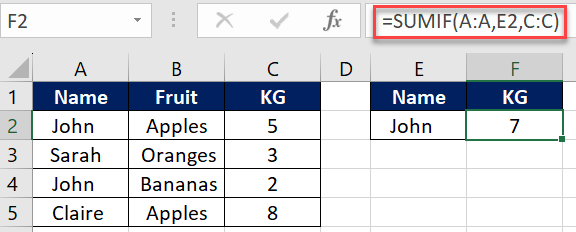
To do this, we can use the SUMIF formula as follows:
=SUMIF(A:A,E2,C:C)
See also: Mastering the Linux Command Line — Your Complete Free Training Guide
This will give us the total sum of all values in column C where the corresponding value in column A is “John”, which is 7 in this case (5+2).
Example 2: Excluding Specific Criteria
Summing values from a column while excluding rows with certain conditions.
Suppose we have a table with the following data and we want to sum the values in column B for all the rows where the value in column A is not equal to “Apples”:
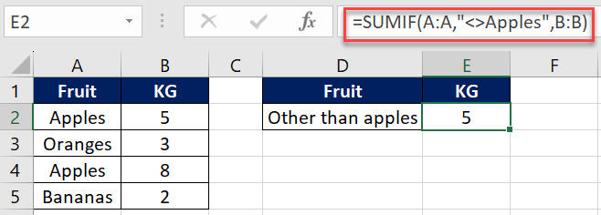
`=SUMIF(A:A,”<>Apples”,B:B)`
This will give us the total sum of all values in column B where the corresponding value in column A is not “Apples”, which is 5 in this case (3+2).
Example 3: Multiple Criteria Summing
Combining criteria to sum values from a column using multiple conditions.
Suppose we have a table with the following data and we want to sum the values in column B for all the rows where the value in column A is equal to “Apples” and the value in column C is greater than 5:
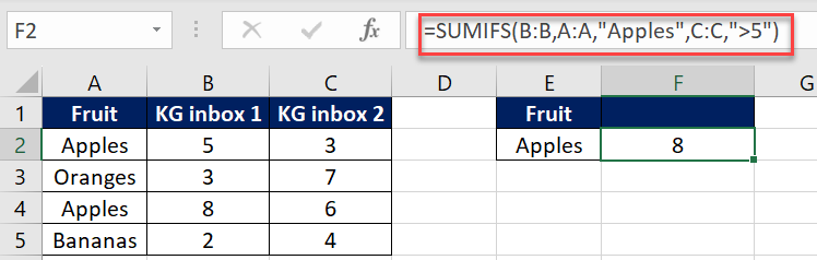
`=SUMIFS(B:B,A:A,”Apples”,C:C,”>5″)`
This will give us the total sum of all values in column B where the corresponding value in column A is “Apples” and the value in column C is greater than 5, which is 8 in this case.
Example 4: Multiple SUMIF Operations
Utilizing SUMIF twice to separately sum values based on different columns’ criteria.
Suppose we have a table with the following data and we want to sum the values in column C for all the rows where the value in column A or column B is equal to “Apples”:
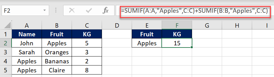
To do this, we can use the SUMIF formula as follows:
`=SUMIF(A:A,”Apples”,C:C)+SUMIF(B:B,”Apples”,C:C)`
This will give us the total sum of all values in column C where the corresponding value in column A or column B is “Apples”, which is 15 in this case.
Example 5: Summing with OR Condition
Adding values based on multiple OR conditions in one column.
Suppose we have a table with the following data and we want to sum the values in column B for all the rows where the value in column A is “Apples” or “Oranges”:

`=SUMIF(A:A,”Apples”,B:B)+SUMIF(A:A,”Oranges”,B:B)`
This will give us the total sum of all values in column B where the corresponding value in column A is “Apples” and “Oranges”, which is 16 in this case.
Example 6: Wildcard Criteria Matching
Using wildcards to match partial string criteria within a column.
Suppose we have a table with the following data and we want to sum the values in column C for all the rows where the value in column A contains “John”:

`=SUMIF(A:A,”*John*”,C:C)`
This will give us the total sum of all values in column C where the corresponding value in column A contains “John”, which is 7 in this case (5+2).
Example 7: Dynamic Date-based Summing
Calculating the sum based on the current date in a specific column.
Suppose we have a table with the following data and we want to sum the values in column B for all the rows where the value in column A is equal to the current date:

`=SUMIF(A:A,TODAY(),B:B)`
This will give us the total sum of all values in column B where the corresponding value in column A is equal to the current date, which will depend on the current date when the formula is calculated.
FAQ about EXCEL sumif function
- What is the syntax of the SUMIF function in Excel?
The SUMIF function syntax is: =SUMIF(range, criteria, [sum_range]).
range: The range to evaluate against the specified criteria. - Can I use multiple criteria with the SUMIF function?
For multiple criteria, you can use the SUMIFS function.
Syntax: =SUMIFS(sum_range, criteria_range1, criteria1, [criteria_range2, criteria2], …). - What types of criteria can be used in the SUMIF function?
Criteria can include numbers, text, wildcards, or logical operators.
Wildcards like asterisk (*) can be used for partial matching. - How does SUMIF differ from SUMIFS?
SUMIF is for a single condition, while SUMIFS handles multiple conditions.
SUMIFS allows more complex criteria combinations. - Can I use cell references as criteria in the SUMIF function?
Yes, you can use cell references as criteria in the SUMIF function.
This allows dynamic adjustments to criteria without modifying the formula.
10 Advanced Excel SUMIFS Function Examples to Boost Your Data Management Skills
7 Common Errors in XLOOKUP and How to Fix Them
2 ways to use XLOOKUP with Multiple Criteria in Excel
Top 8 Powerful Excel XLOOKUP Examples: Enhance Your Data Analysis Skills
Return All Matches in Excel Using XLOOKUP and Other Functions