Top 8 Powerful Excel XLOOKUP Examples: Enhance Your Data Analysis Skills

XLOOKUP is a powerful function introduced in Excel to simplify and enhance the capabilities of searching and retrieving data from a range or array.

It’s designed to replace older functions like VLOOKUP, HLOOKUP, and LOOKUP by offering more flexibility and ease of use.

Features of XLOOKUP

Lookup Value Flexibility:

XLOOKUP can find values both vertically and horizontally, eliminating the need for separate VLOOKUP and HLOOKUP functions.

Return Array:

It allows you to specify a return array from where the matching result is fetched, which can be different from the lookup array.

Default Value for Not Found:

XLOOKUP can return a default value or message when the lookup value is not found, improving error handling over VLOOKUP’s error messages.

Search Mode Options:

It includes options for different search modes, such as searching from top to bottom, bottom to top, binary search for sorted data, and more.

Support for Wildcards:

XLOOKUP supports the use of wildcards (*, ?) for partial text matches, making it versatile for various text search scenarios.

Simpler, More Readable Syntax:

XLOOKUP’s syntax is more straightforward and intuitive compared to its predecessors.

Syntax of XLOOKUP

XLOOKUP(lookup_value, lookup_array, return_array, [if_not_found], [match_mode], [search_mode])

• lookup_value: The value to search for.
• lookup_array: The array or range to search.
• return_array: The array or range from which to return a value.
• [if_not_found]: (Optional) The value to return if the lookup_value is not found. Defaults to #N/A.
• [match_mode]: (Optional) Specifies the match type: exact match (0), exact match or next smaller item (-1), wildcard match (2). Default is 0.
• [search_mode]: (Optional) Specifies the search mode: search first-to-last (1), search last-to-first (-1), binary search ascending (2), binary search descending (-2). Default is 1.

 

Vertical lookup using XLOOKUP

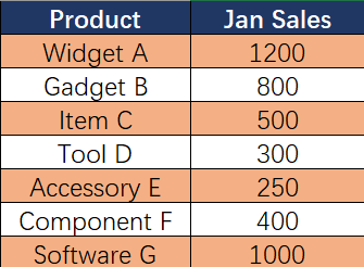
Example Data:

Suppose we have the following data in an Excel sheet:

Objective:

Find the price of the product “Accessory E”.

XLOOKUP Formula:

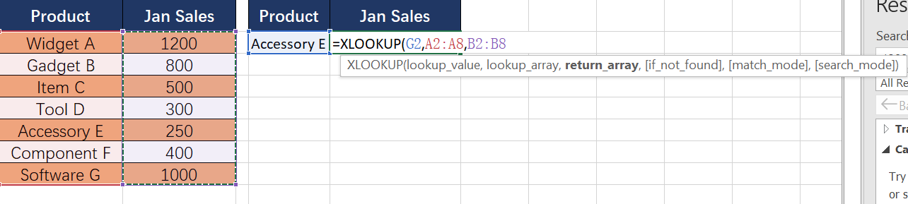
To achieve this, we would use the XLOOKUP function as follows:

=XLOOKUP(G2,A2:A8,B2:B8)

Breakdown of the Formula:

• G2:This is our lookup value. We are searching for the price of “Accessory E”.
• A2:A8: This is our lookup array. XLOOKUP will search for the “Accessory E” within this range.
• B2:B8: This is our return array. Once XLOOKUP finds “Accessory E” in the lookup array, it will return the corresponding value from this range.

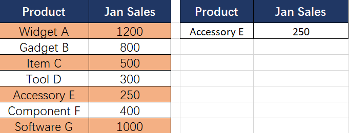
Result:

When you input this formula into a cell, it will return 250, which is the Jan Sales of the “Accessory E”.

Explanation:

The XLOOKUP function looks through the range A2:A8 to find the value “Accessory E”. Once found, it returns the corresponding value from the same row in the range B2:B8, which is the Jan Sales of the product.

Horizontal lookup using XLOOKUP

Example Data:

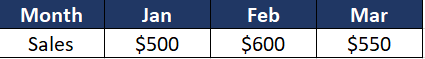
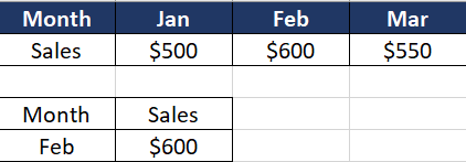
Suppose we have sales data for the first quarter of the year laid out as follows:

Objective:

Find the sales figure for the month of February.

XLOOKUP Formula:

The formula to find February’s sales would be:

=XLOOKUP("Feb", A1:D1, A2:D2)

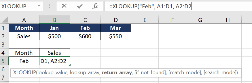
Breakdown of the Formula:

• “Feb”: This is the lookup value, representing the month we’re searching for.
• A1:D1: This is the lookup array, where XLOOKUP will search for the month “Feb”.
• A2:D2: This is the return array. Once XLOOKUP finds “Feb” in the lookup array, it will return the corresponding value from this row, which in this case is the sales figure for February.

Result:

Entering this formula in a cell will return $600, which is the sales figure for the month of February.

Explanation:

This example demonstrates a horizontal lookup using XLOOKUP, which is especially useful for datasets where data points are laid out in a row.

The function efficiently searches across the specified row to find the matching month and then returns the corresponding sales figure from the same position in the second row.

Exact Match

Example Data:

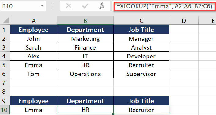
Let’s consider a scenario where we have a dataset of employees with their respective departments and job titles in an Excel sheet:

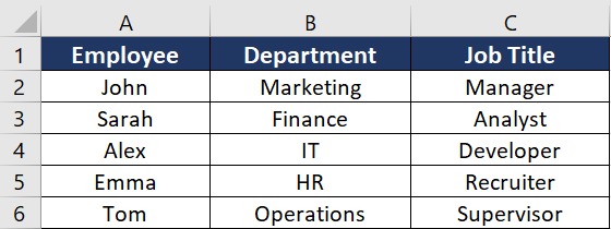
Objective:

Find both the department and job title for a specific employee, say “Emma”.

XLOOKUP Formula:

To achieve this, you would use the XLOOKUP function as follows:

=XLOOKUP("Emma", A2:A6, B2:C6)

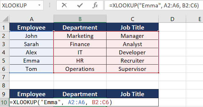
Breakdown of the Formula:

• “Emma”: This is our lookup value. We are searching for information related to “Emma”.
• A2:A6: This is our lookup array. XLOOKUP will search for “Emma” within this vertical range in Column A.
• B2:C6: This is our return array. Once XLOOKUP finds “Emma” in the lookup array, it will return the corresponding values from both Columns B and C.

Result:

When you enter this formula into a cell, it will return both “HR” and “Recruiter”, which are the department and job title of “Emma”, respectively.

Explanation:

This example demonstrates the use of XLOOKUP to return multiple values corresponding to a single lookup value. By setting the return array to span multiple columns (B2:C6 in this case), XLOOKUP can fetch and display more than one related piece of data.

This is particularly useful when you need to retrieve several pieces of related information from a dataset, like details from a record or multiple attributes associated with a single entity, without having to use multiple lookup formulas.

If Not Found

Example Data:

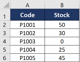
Imagine we have an Excel sheet with a list of product codes and their corresponding stock levels:

Objective:

Find the stock level for a specific product code. If the product code does not exist in the list, return a message saying “Not Found”.

XLOOKUP Formula:

To achieve this, you would use the XLOOKUP function as follows, assuming the product code you’re looking for is in cell A2:

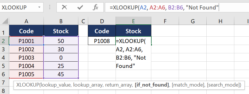
=XLOOKUP(D2, A2:A6, B2:B6, "Not Found")

Breakdown of the Formula:

• D2: This is our lookup value, which is the product code we’re searching for.
• A2:A6: This is our lookup array. XLOOKUP will search for the value in A2 within this vertical range in Column A.
• B2:B6: This is our return array. Once XLOOKUP finds the value from A2 in the lookup array, it will return the corresponding value from Column B.
• “Not Found”: This is the default value that XLOOKUP will return if the lookup value is not found in the lookup array.

Result:

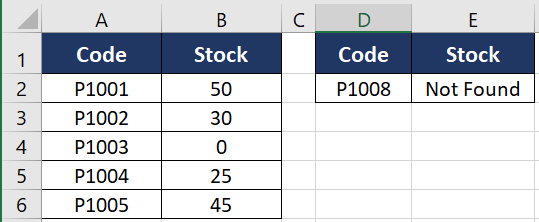
If you enter a product code in cell D2 and execute this formula, it will return the stock level for that product. However, if the product code in D2 does not exist in the range A2:A6, the formula will return “Not Found”.

Explanation:

This example illustrates how XLOOKUP can be used for error handling in scenarios where the lookup value might not always be present in the data set.

The addition of the “Not Found” parameter in the formula provides a user-friendly way to handle such cases, making the function more robust and the data output clearer in situations where the search criteria aren’t met.

Wildcard Search

Example Data:

Let’s consider an Excel sheet with a list of product names and their corresponding prices:

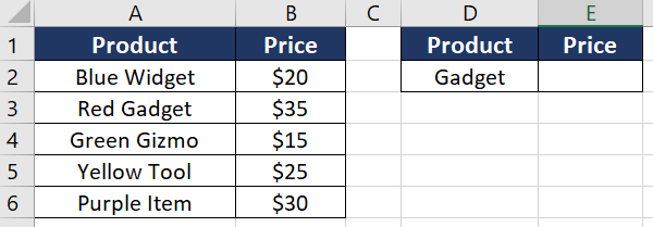
Objective:

Find the price of a product where the name contains a specific keyword, regardless of its position in the product name. For example, find the price of a product containing the word “Gadget”.

XLOOKUP Formula:

Assuming you have the keyword in cell A2 (“Gadget” in this case), the formula would be:

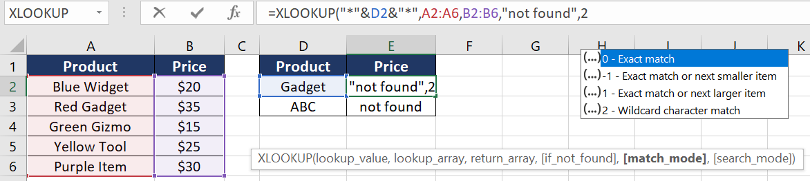
=XLOOKUP("*"&D3&"*",A3:A7,B3:B7,"not found",2)

 

Breakdown of the Formula:

• “*”&D3&”*”:This creates a search pattern combining the wildcard characters * with the value in A2. The * wildcard matches any sequence of characters, so this pattern will match any text that includes the value in A2.
• A2:A6: This is the lookup array where the function searches for the pattern.
• B2:B6: This is the return array from which the function retrieves the corresponding value.

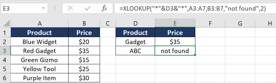
Result:

If “Gadget” is entered in A2, the formula will return $35, which is the price of the “Red Gadget”.

Explanation:

The wildcard search in XLOOKUP is useful for finding a match in cases where the exact text of the lookup value might be part of a larger string.

By using the * character before and after the value in D2, the function will search for any occurrence of that value within the strings in the lookup array (A2:A6 in this example).

This feature is especially helpful in scenarios like searching within product names, descriptions, or any data where the exact position of the lookup value within the text is unknown or variable.

It provides a flexible and powerful way to perform partial text searches in Excel datasets.

Case-Insensitive Search

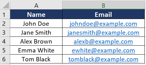
Example Data:

Consider an Excel sheet that contains a list of employee names and their corresponding email addresses:

Objective

Find the email address of an employee when the name is entered, ensuring that the search is not affected by the case (uppercase/lowercase) of the letters.

XLOOKUP Formula

If you want to search for an employee’s name entered in cell A2 (e.g., “john doe”, “John Doe”, “JOHN DOE”, etc.) and retrieve their email, the formula would be:

=XLOOKUP(LOWER(D2), LOWER(A2:A6), B2:B6)

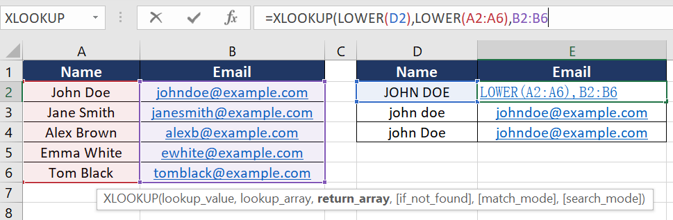
Breakdown of the Formula:

• LOWER(D2): This function converts the lookup value in D2 to lowercase. It ensures that the search is case-insensitive by standardizing the case of the input.
• LOWER(A2:A6): This function converts all the values in the lookup array (A2:A6, the names of the employees) to lowercase. It matches the standardization done to the lookup value.
• B2:B6: This is the return array from which the function retrieves the corresponding email address.

 

Result:

If “John Doe” is entered in D2 in any letter case (like “john doe” or “JOHN DOE”), the formula will correctly return [email protected].

Explanation:

XLOOKUP, by default, performs case-sensitive searches. However, in many scenarios, especially when dealing with names, email addresses, or text data, a case-insensitive search is more practical.

By using the LOWER function on both the lookup value and the lookup array, the formula ensures that the search is not affected by the letter case. This approach standardizes all text to lowercase, making the search uniform and thereby case-insensitive.

Two-Way Lookup

Example Data:

Let’s say you have an Excel sheet that contains a matrix of data representing sales figures of various products across different months.

Data Layout:

Objective:

You want to find the sales figure for a specific product in a specific month. For example, you might want to know the sales of “Gadget” in “Mar”.

XLOOKUP Formula:

To achieve this, you can set up a two-way lookup using XLOOKUP. Assuming A2 contains the product name “Gadget” and B2 contains the month “Mar”, the formula would be:

=XLOOKUP(H2,A2:A5,XLOOKUP(I1,B1:F1,B2:F5))

 

 

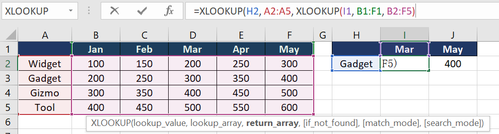
Breakdown of the Formula:

• H2: This cell contains the lookup value for the product name (e.g., “Gadget”).
• A2:A5: This range contains the list of product names to match with A2.
• I1: This cell contains the lookup value for the month (e.g., “Mar”).
• B1:F1: This range contains the months to match with B2.
• B2:F5: This is the matrix containing the sales data. The nested XLOOKUP will return a single row from this matrix corresponding to the product found in the first XLOOKUP.
• The outer XLOOKUP then looks across this row to find the sales figure for the specified month.

Result:

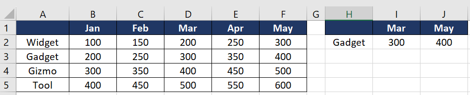
Upon entering “Gadget” in H2 and “Mar” in I2, the formula returns 300, which is the sales figure for “Gadget” in the month of “Mar”.

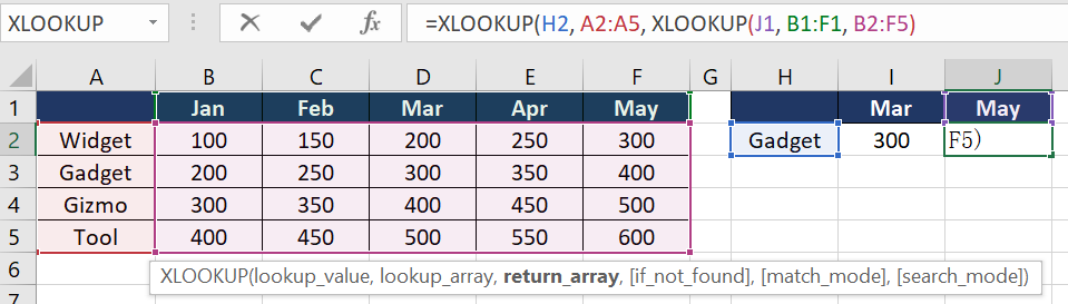
Explanation:

This example illustrates a two-way lookup using XLOOKUP, which is particularly useful for searching within a matrix or a grid-like data structure.

The first XLOOKUP searches vertically for the product and returns an entire row of sales figures. The second, nested XLOOKUP then searches horizontally within this returned row to find the sales figure for the specified month.

This two-way or matrix lookup capability of XLOOKUP is extremely powerful for cross-referencing data across both rows and columns, making it a valuable tool for more complex data retrieval tasks in Excel.