Return All Matches in Excel Using XLOOKUP and Other Functions

While XLOOKUP in Excel is primarily designed to return the first match, it can be combined with other functions like FILTER or TEXTJOIN, or used with an array formula to return all matches for a given criterion.

XLOOKUP Returns the First Match in Excel

This is an example to demonstrate how XLOOKUP in Excel is used to find and return the first match it encounters in a given range.

Scenario: Finding the Price of a Product

Consider a scenario where you have a list of products with their prices, and you want to find the price of a specific product, “Apple”, which appears multiple times with different prices.

Table Example:

Product	Price
Apple	$1
Banana	$2
Apple	$1.5
Orange	$1.75
Apple	$1.25

Objective:

Find the price of an “Apple” using XLOOKUP.

XLOOKUP Formula:

=XLOOKUP("Apple", A2:A6, B2:B6)

Explanation:

• Lookup Value: “Apple” – The value you are searching for.
• Lookup Array: A2:A6 – The range where the search is performed.
• Return Array: B2:B6 – The range from which the corresponding value is returned.

The formula searches for the first “Apple” in A2:A6 and returns its price from B2:B6, which is $1 in this case.

Method 1: Using FILTER Function to Return All Matches

If you have Excel for Microsoft 365 or Excel 2021, which supports dynamic arrays, you can use the FILTER function.

It can be used to return all matching entries from a range based on specified criteria. This method is especially useful for extracting a list of values that meet certain conditions without needing to write complex formulas.

=FILTER(ReturnRange, CriteriaRange = Criteria)

Example:

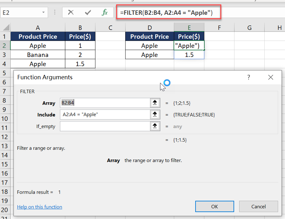
Consider a list of products and prices. To find all prices for “Apple”, the formula would be:

=FILTER(B2:B4, A2:A4 = "Apple")

This returns all prices for “Apple”, both $1 and $1.5.

Method 2: Using TEXTJOIN and Array Formula to Return All Matches

In versions of Excel that do not support dynamic arrays, combining TEXTJOIN with an array formula offers a way to concatenate all matching values into a single string.

=TEXTJOIN(", ", TRUE, IF(CriteriaRange = Criteria, ReturnRange, ""))

=TEXTJOIN(", ", TRUE, IF(A2:A4 = "Apple", B2:B4, ""))

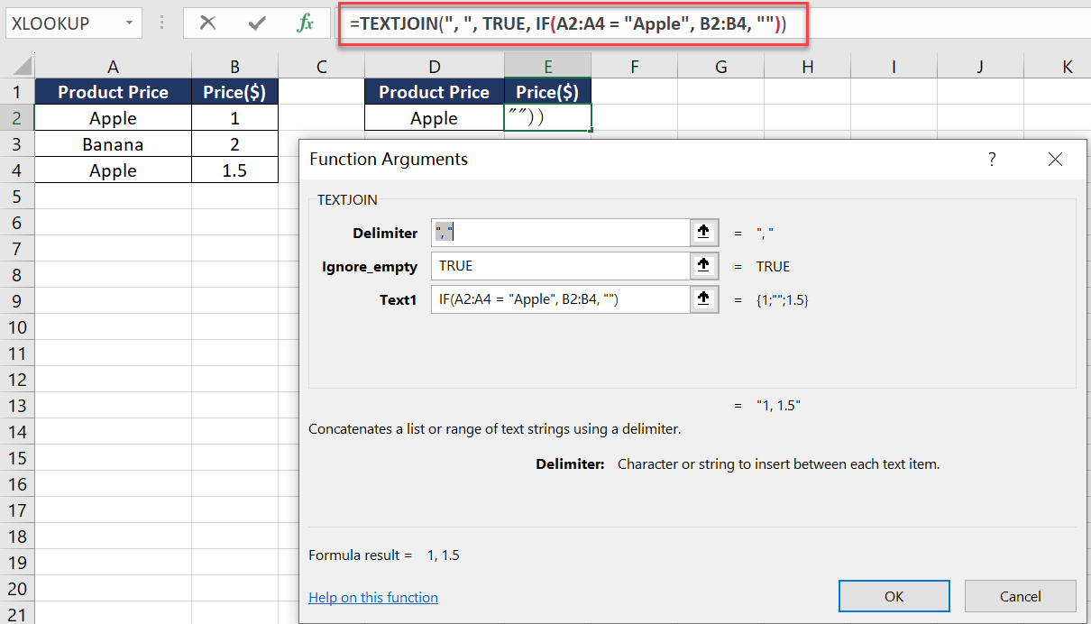
Press Ctrl + Shift + Enter after typing this formula. It concatenates all prices for “Apple” into a single string, resulting in “1, 1.5”.

Conclusion:

• The FILTER method is more straightforward but requires Excel that supports dynamic arrays.
• The TEXTJOIN method works in older versions of Excel but concatenates the results into a single string.
• Both methods are useful for different scenarios, depending on the Excel version and the desired output format.

These methods effectively expand the functionality of XLOOKUP in Excel, allowing for the retrieval of all matches for a given criterion.