Table of Contents
LEFT function – extract a specified number of characters from the left side of a text string
The LEFT function in Excel is used to extract a specified number of characters from the left side of a text string. It’s particularly helpful when you need to parse or work with a portion of text.
The syntax for the LEFT function is:
=LEFT(text, [num_chars])
- text: The original text string from which you want to extract characters.
- num_chars: The number of characters you want to extract from the left side of the text string. This parameter is optional. If omitted, it defaults to 1.
Example, suppose cell A1 contains the text “Excel is awesome”. You can use the LEFT function to extract the first five characters:
=LEFT(A1, 5)
This formula will return “Excel”, which is the first five characters from the left side of the text in cell A1.
Example: Suppose you have a list of full names in a column, and you want to extract only the first name from each name.
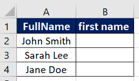
To extract the first name using the LEFT function, you would use the following formula in cell B2:
=LEFT(A2,FIND(" ",A2)-1)
See also: Mastering the Linux Command Line — Your Complete Free Training Guide
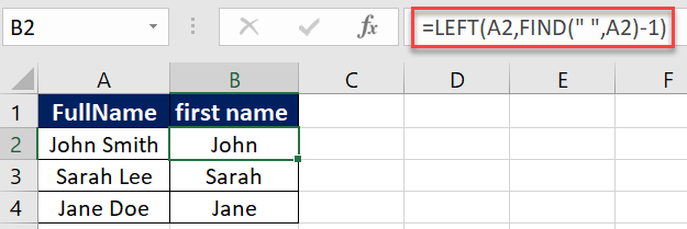
Explanation: The formula uses the FIND function to locate the space character in the full name, and then subtracts 1 from its position to extract only the first name from the left.
MID Function – extract a specific number of characters from a text string in Excel
The MID function is used to extract a specific number of characters from a text string in Excel. The syntax for the MID function is as follows:
=MID(text, start_num, num_char)
Where ‘text’ is the text string from which you want to extract characters, ‘start_num’ is the position where you want to start extracting characters, and ‘num_char’ is the number of characters to extract.
Example:
=MID("Excel is powerful", 7, 2)
This formula extracts 2 characters starting from the 7th position in the text, resulting in “is”.
Example: Using Cell References
=MID(A1, 3, 4)
If cell A1 contains “Data Analysis”, this formula extracts 4 characters starting from the 3rd position, resulting in “ta A”.
Example: Dynamic Length Determination
=MID(B1, FIND(" ", B1) + 1, LEN(B1))
If cell B1 contains “Data Analysis in Excel”, this formula extracts text after the first space, resulting in “Analysis in Excel”.
Example: Extracting Phone Numbers
=MID(C2, FIND("-", C2) + 1, 3)
If cell C2 contains “123-456-7890”, this formula extracts the 3 characters following the first hyphen, resulting in “456”.
Example: Suppose you have a list of email addresses in a column, and you want to extract only the domain name from each address.
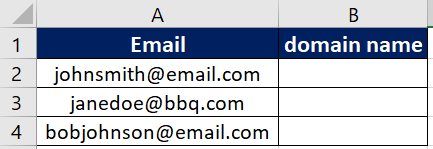
To extract the domain name using the MID function, you would use the following formula in cell B2:
=MID(A2,FIND("@",A2)+1,LEN(A2))
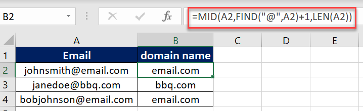
Explanation: The formula uses the FIND function to locate the “@” symbol in the email address, and adds 1 to its position to start extracting characters from the right of the symbol. The formula then uses the LEN function to determine the total length of the remaining characters to extract.
RIGHT Function – extract the rightmost characters from a text string in Excel
The RIGHT function is used to extract the rightmost characters from a text string in Excel. The syntax for the RIGHT function is as follows:
=RIGHT(text, num_char)
Where ‘text’ is the text string from which you want to extract characters, and ‘num_char’ is the number of characters to extract from the right side of the string.
Example:
=RIGHT("Hello, World!", 6)
This formula extracts the last 6 characters from the text, resulting in “World!”.
Example: Dynamic Length Determination
=RIGHT(B1, LEN(B1) - FIND(",", B1))
If cell B1 contains “Software Engineering, IT Sector”, this formula extracts text after the comma, resulting in ” IT Sector”.
Example: Extracting File Extensions
=RIGHT(C2, LEN(C2) - FIND(".", C2))
If cell C2 contains “document.docx”, this formula extracts the file extension, resulting in “docx”.
Example: Suppose you have a list of phone numbers in a column, and you want to extract only the last four digits from each number.

To extract the last four digits using the RIGHT function, you would use the following formula in cell B2:
=RIGHT(A2,4)
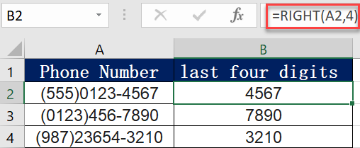
Explanation: The formula simply uses the RIGHT function to extract the last four characters from each phone number.
In conclusion, the LEFT, MID, and RIGHT functions are essential tools in Excel for extracting specific pieces of data from larger sets. By understanding how to use these functions, you can streamline your data analysis and make your work more efficient.