3 easy ways to Alternate row colors in Excel

Alternate row color shading in Excel, also known as “zebra striping,” refers to the practice of formatting rows in a spreadsheet so that adjacent rows have different background colors.

This visual distinction makes data easier to read and scan, especially in large spreadsheets with numerous rows of information.

In this article, we will introduce 3 different ways to alternate row colors in Excel.

Apply row color shading in Excel using predefined table styles

Predefined table styles in Excel are a set of built-in, ready-to-use table formats that you can apply to your data tables.

These styles provide a quick and efficient way to make your tables look more professional and visually appealing. They are particularly useful for enhancing the readability and presentation of your data.

To apply row shading in Excel using predefined table styles, follow these steps:

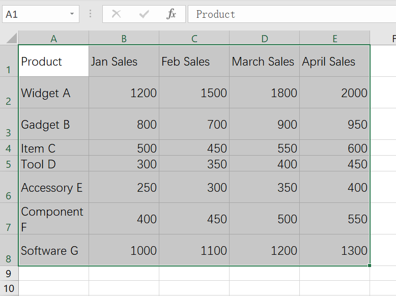
1. Select Your Data:
   • Click on the first cell of your data set.
   • Drag to select the entire range you want to format. You can also select entire rows or columns by clicking on their headers.
     
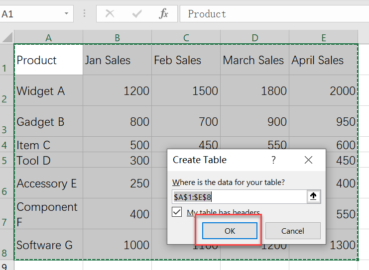
2. Convert Data to a Table:
   • Go to the ‘Home’ tab on the Excel ribbon.
   • Click ‘Format as Table’ in the ‘Styles’ group.
     
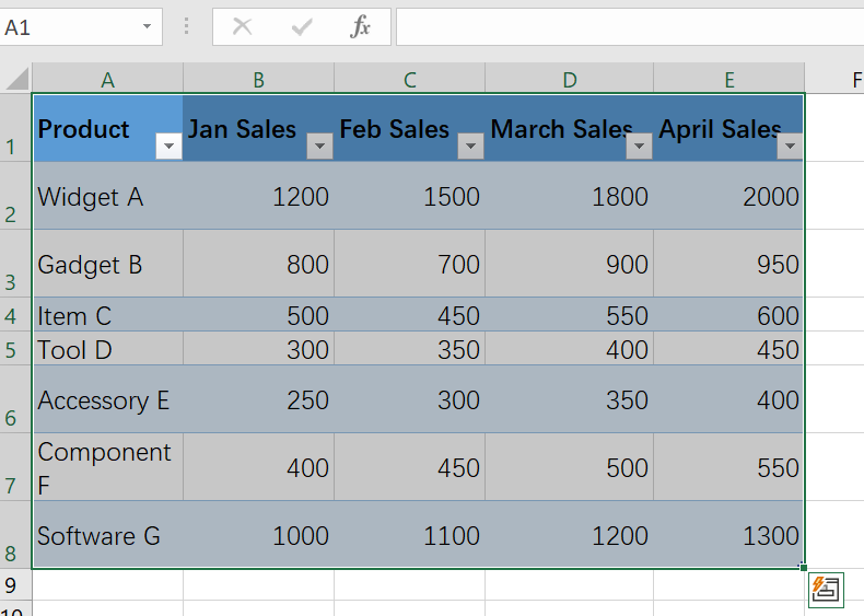
3. Choose a Table Style:
   • A gallery of table styles will appear.
   • Hover over the styles to preview them on your data.
   • Click on the style you prefer. Styles with alternate row shading are easily identified by their preview.
     
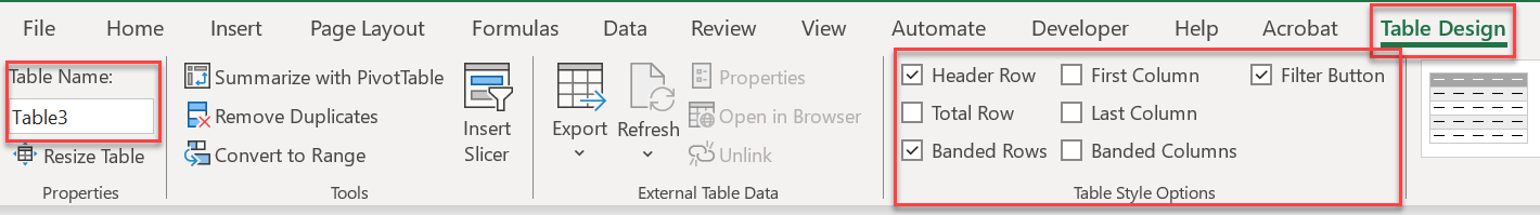
4. Adjust Table Settings and Refine the Table (Optional):
   • Once the table style is applied, a ‘Table Tools Design’ tab will appear.
   • Use this tab to further customize your table.
   • You can check or uncheck options like ‘Header Row’, ‘Total Row’, ‘Banded Rows’, etc., according to your preferences.
   • You can adjust the table range by dragging the handles at the table’s corners.
   • If necessary, rename the table for easier reference in formulas. Do this in the ‘Table Tools Design’ tab, in the ‘Properties’ group.
     
5. Additional Formatting (Optional):
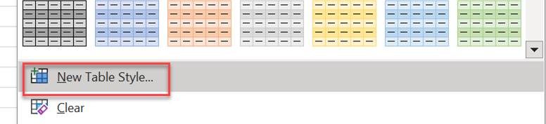
   • For further customization, right-click on the table and choose ‘Table Styles’.
   • Select ‘New Table Style’ for more advanced options, like modifying specific elements of the table style.
     

Note: This method not only improves the visual organization of your data but also comes with additional table functionalities like sorting and filtering.

Apply alternate row color shading in Excel using conditional formatting

Conditional formatting in Excel is a powerful feature that allows you to apply specific formatting to cells based on certain criteria or conditions.

This means that the appearance of a cell (like its color, font style, or border type) can automatically change depending on the cell’s value or the value of another cell.

It’s a great tool for visually emphasizing key information, identifying trends, or highlighting anomalies in your data.

To apply alternate row color shading in Excel using conditional formatting, follow these instructions:

1. Select Your Data Range:
   • Click the first cell in your dataset.
   • Drag to highlight the entire area you want to format. Alternatively, click the row numbers to select entire rows.
     
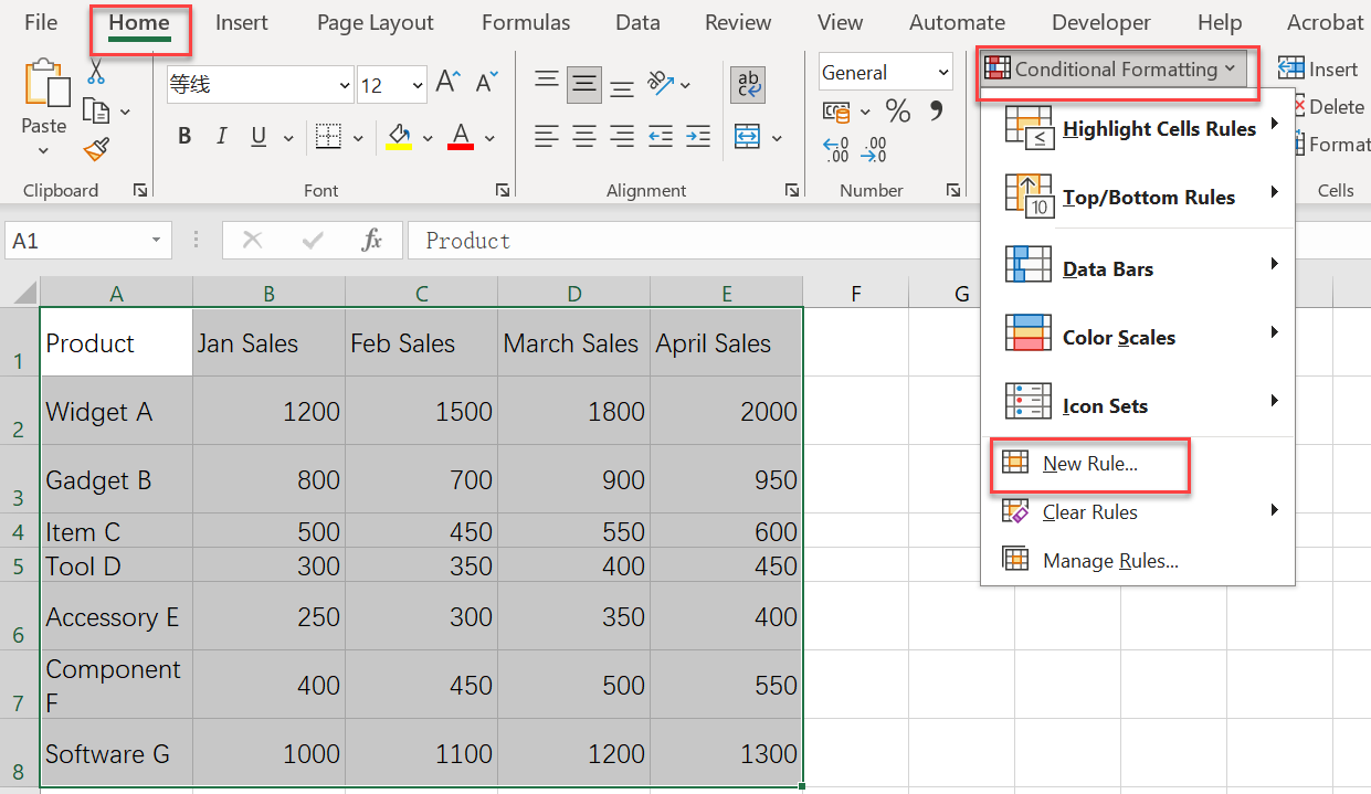
2. Access Conditional Formatting:
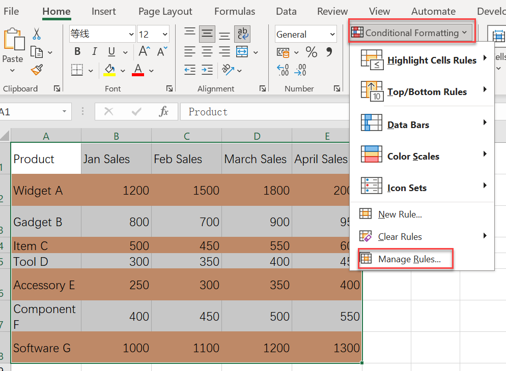
   • Navigate to the ‘Home’ tab on the ribbon.
   • Click ‘Conditional Formatting’ in the ‘Styles’ group.
     
3. Create a New Formatting Rule:
   • Select ‘New Rule’ from the Conditional Formatting dropdown.
     
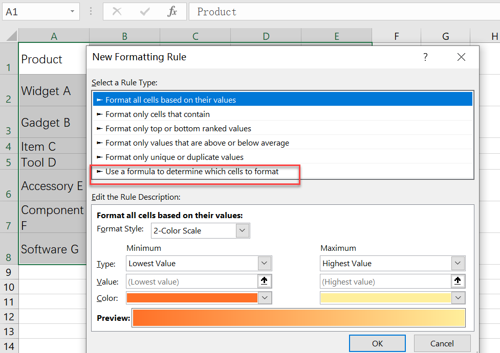
4. Choose to Use a Formula:
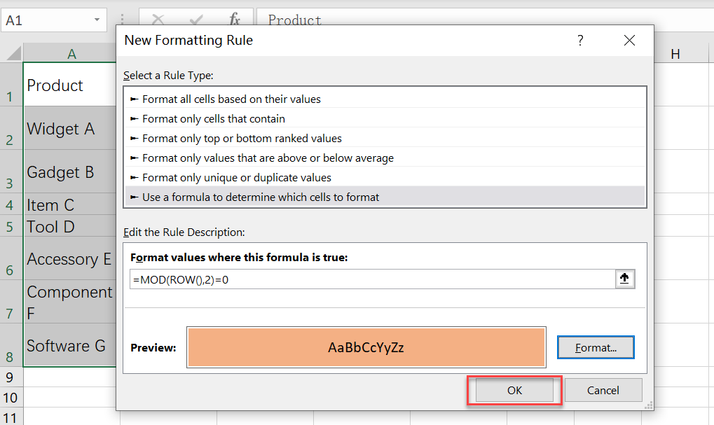
   • In the New Formatting Rule dialog, choose ‘Use a formula to determine which cells to format’.
     
5. Input the Formula for Alternate Shading:
   • Type in =MOD(ROW(),2)=0 to shade even rows, or =MOD(ROW(),2)=1 for odd rows.
   • This formula checks if a row number is even or odd and applies the format accordingly.
     
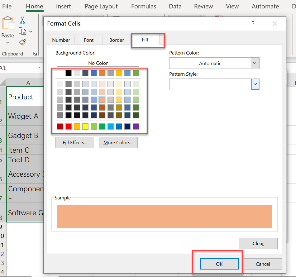
6. Define the Format:
   • Click the ‘Format’ button.
   • Select your preferred fill color for the shading under the ‘Fill’ tab.
   • You can also alter text formatting here, if desired.
   • Click ‘OK’ to close the Format Cells window.
     
7. Apply the Rule:
   • Click ‘OK’ in the New Formatting Rule dialog to apply your conditional formatting.
     
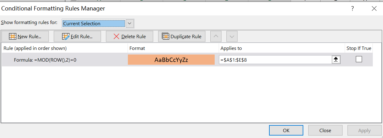
8. Modify the Range if Needed:
   • If you need to change the range later, go to Conditional Formatting → Manage Rules. Here, you can edit the range or modify the rule.
     

 

Apply alternate row color shading in Excel using office script

Office Script is a feature in Microsoft Excel that’s part of the Office 365 suite. It allows you to automate tasks and workflows in Excel, similar to how VBA (Visual Basic for Applications) works, but with some key differences.

Office Scripts is designed with modern cloud-based environments in mind, offering a more accessible and user-friendly approach to automation in Excel.

We can also use Office Script to add colors to each row in an Excel worksheet, with odd rows colored yellow and even rows colored white.

Here’s a script that will do just that:

async function main(workbook: ExcelScript.Workbook) {
  let selectedSheet = workbook.getActiveWorksheet();

  // Get the used range of the worksheet
  let usedRange = selectedSheet.getUsedRange();

  // Get the total number of rows in the used range
  let totalRows = usedRange.getRowCount();

  // Loop through each row
  for (let i = 0; i < totalRows; i++) {
    // Get the current row
    let row = usedRange.getRow(i);

    // Check if the row number is odd or even
    if (i % 2 === 0) {
      // Even row - set the color to white
      row.getFormat().getFill().setColor("white");
    } else {
      // Odd row - set the color to yellow
      row.getFormat().getFill().setColor("yellow");
    }
  }
}

To use this script:

• Open your Excel workbook.
• Go to the “Automate” tab and select “New Script.”
• Paste the script into the script editor.
• Save the script.
• Run the script to apply the color formatting to your worksheet.
• This script will color each row in the used range of your active worksheet. Odd rows will be colored yellow and even rows will be colored white.

 

Best Practices

Choose Colors Wisely: Ensure that the colors used are distinct enough to make a difference but not too harsh on the eyes.
Keep Consistency: If you’re using multiple sheets or tables, maintaining a consistent color scheme helps in keeping the data presentation uniform.

By following these steps, you’ll have neatly shaded alternate rows in your Excel sheet, enhancing readability and visual appeal. Hope you like it.